Part 1:
Trigonometry
In its simplest definition, trigonometry is the study of
the ratios of various sides in a right triangle. Recall the mnemonic “SOHCAHTOA”, which helped you remember that
the sine of a given angle is the ratio of length of the side opposite the angle
to the length of the hypotenuse of the triangle.
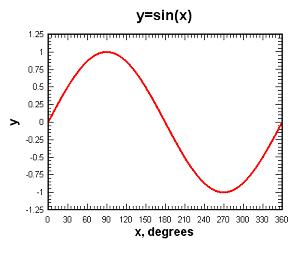
Let’s consider the sin value of a few important angles from 0 to 360 degrees:
Sin(0) = 0
Sin(90) = 1
Sin(180) = 0
Sin(270) = -1
Sin(360) = 0
You can plot these values on a
Cartesian XY plane, with the angle on the x-axis, and the sin value on the
y-axis. When you plot the sin value of
every degree from 0 to 360, including the ones listed above, you get this graph:
What do this have to do with computer animation? Well, we wanted to make something that resembled liquid
sloshing around in a crystal ball. If
you plot
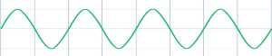
y = sin(x) you get that simple sine wave. In the next diagram, we are plotting sin(x) well past 360
degrees. As you can see, the values
start to repeat themselves after you pass 360 (and 720, 1080, etc). This is because a 361 degree angle shares
certain characteristics with a 1 degree angle.
Of course, if we merely plotted this curve, it would just be static and
uniform, and the “water” wouldn’t even be moving. To animate the water, we need to repeatedly plot variations of
this curve (frames). To do this, we
introduced a variable t which increases on every frame, and plotted y=sin(x+t). For each cycle, you get the
same basic sine wave, except it slides left a little bit each time, as t increases.
This happens because the +t has the effect of increasing the angle value
whose sin we are calculating. Likewise,
plotting y = sin(x-t) would slide it to the right.
This still does not look like water, however. It just looks like a uniform sin curve sliding across the screen. To look like real liquid, we need some more randomness and
variety! Recall that the frequency of a sin
curve indicates how quickly it completes the full cycle from Figure 1. The higher the frequency, the more often it
repeats in a given interval.
(Note: In radio transmission,
FM stands for “frequency modulation” of the sound waves, and AM stands for
“amplitude modulation”, or the height of the curve.)
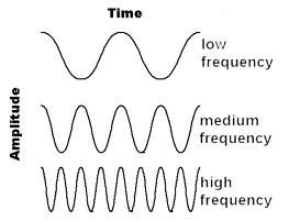
So, if you vary the frequency of the sine wave, you will get more
variation in the curve.
Y = sin((x + t)
* freq) will produce sine waves with different periods, still rolling to the
left because of the +t (rolling at the freq scaled rate).
Further, you can even plot the sum of 2 different sine waves. This is where it gets interesting!
Y = sin((x + t + phase_offset) * f1) + sin((x - t) * f2)
yields a more complex
roiling surface than a simple sliding sine wave.
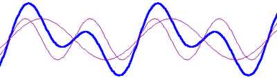
The dark curve is the sum of the 2 lighter sine waves, and will be the
“water”. The most important part is
that the 2 sine waves are rolling in opposite directions, (notice the –t
in the 2nd sin term) and the shape of their sum is always
changing. In addition, we randomly jitter f1 and f2 up and down a bit, as
well as jittering the phase offset, in order to reduce visual
repetitiveness. This really starts to
look like gurgling water!
To
really internalize this concept, you need to see the animation in action.
Click here, and toggle the settings until the "Aha!" moment
Part 2: Calculus
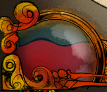
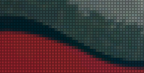
Below is a screen shot of game where we implemented the wave-like liquid
conceived in Part 1. The red liquid and
adjacent black line are generated dynamically, and then the crystal ball
container image is drawn over it, with alpha blending. The wave motion is
generated by running 3 rolling sine waves at different frequencies and adding
them together.
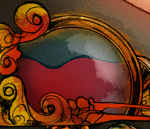
As you can see, there is some noticeable stair-stepping
jaggedness.

This happens because the line described by our sum-of-sines
function is infinitely thin, but the pixels are not.
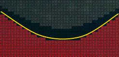
Is there a way to make the transition from black to red a
little smoother? Right now, each pixel
is either entirely black or red. The
jaggedness could be smoothed, to some degree, if we colored some of the pixels
a blended shade of red and black. To
determine how to shade, let’s take a closer look at one of these “transition”
pixels.
The pixels on the borderline of the red and black sections have the sin curve going through
them. For each pixel, the way the curve
goes through it can determine how to shade these pixels.
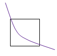
To accurately determine what percentage should be weighted
red vs. black, we need to find the area under the line and dividing by the area
of the pixel. In other words, determine
what percentage of the pixel is over and under the curve.
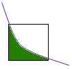
You can only have one color for a given pixel, of
course. But, if you figured out that 17% of a pixel is under the curve
(color1 - red) and the remaining 83% is above the curve (color2 - black), you
can use that ratio as a blending factor to mix the red and black, for that
pixel:
pixel.r = color1.r * 0.17 + color2.r * 0.83;
pixel.g = color1.g* 0.17 + color2.g * 0.83;
pixel.b = color1.b * 0.17 + color2.b * 0.83;
Well then, the thousand dollar question is: How do you find the area under a curve? Answer: Integral Calculus! The area under a sin curve is calculated with the following indefinite integral:
Integrating our sum-of-sines curve is a little more complex:
For each pixel, we integrated the sum-of-sines, and then
divided by the area of the pixel to determine the blending factor. We present a side-by-side comparison below. As you can see, the jagged edges are much smoother now!
Before
After
Before
After